For many designers it might not be clear when it makes sense to use a nonlinear solver versus a linear solver. The truth is ALL studies can be run using nonlinear. The reason we don’t always use it is because it takes several times longer to solve. Many times linear static will provide valid results and solves very quickly.
So what are the situations where linear static studies are not a good fit? Here are a few reasons to use nonlinear. We will illustrate one example in this article.
- Higher accuracy
- Displacements are large in comparison to the model dimensions
- Material stress/strain curve is nonlinear (Rubbers, Plastic)
- Complex loading conditions
- Contact stresses between components (Included with Inventor Professional)
- Geometric conditions
- Post yield behavior
- Buckling (Change in stiffness during loading)
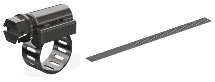
Let’s take a look at large displacements using a hose clamp. The material starts out as a flat piece of sheet metal before being bent 360 degrees. How much force does it take to bend it all the way around? The general rule is the displacement should be less than 5% of the overall size of the model in order to maintain confidence in linear static results. In this example the displacement is several times the size of the part!
“The rule makes sense. But I still don’t know why it has to be run nonlinear??”
Basically speaking, the linear static study applies the entire load in one shot. The direction of the load doesn’t change as it is applied and the stiffness of the model is assumed to be about the same before and after the full load. With the hose clamp the direction of the load is constantly changing and it gets significantly stiffer as it is bent all the way around.
Since the hose clamp is made of metal it is also yielding. That’s why the clamp doesn’t bounce back to the flattened state after it is bent. There is residual stress and displacement when the load is released. And here is the good news. Nonlinear studies can measure that too!
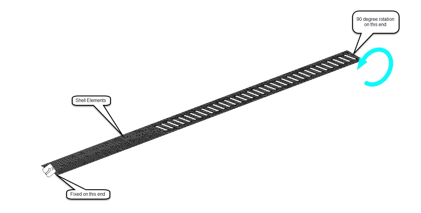
Let’s begin by running the linear static study. We will use shell elements which will solve faster and provide more accuracy due to bending. Then it is fixed on one end. And finally there is a prescribed rotation of 90 degrees on the other end.
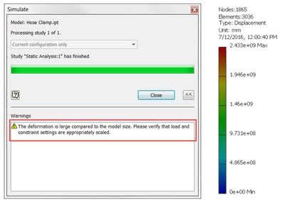
When running the solver, you may be presented with a friendly warning. “The deformation is large compared to the model size”.
The result value for maximum displacement is huge! In this study we are observing 2,400 kilometers! This is a classic limitation for linear static studies. The initial stiffness of the model is very low in the direction of the load. As the rotation is applied the stiffness increases greatly, and linear static studies don’t account for that.
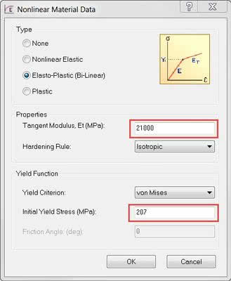
Now let’s run this as a nonlinear study using a similar setup. We will make one change to the material. In the linear study we used Elastic Modulus for the stress/strain curve. This time we will include the Tangent Modulus which is the new stress/strain after the material has yielded. Which does occur with the hose clamp. In this case the Tangent Modulus is 10% of the Elastic Modulus. In other words, the material is softening after it yields.
The constraints will remain the same. We will change the load to rotate the end a full 360 degrees. Now we are ready to run the nonlinear solver!
To put it simply the load or prescribed displacement in this case is applied in increments or time steps. The user has the flexibility to decide how many increments to calculate. In between each increment the stiffness of the model is updated before calculating the next time step. The stiffness may increase or suddenly decrease in the case of buckling or loss of stability.
After running the solver, we now have a much more accurate representation of the behavior of the model. We can even animate it to understand how it works. We can see the slots for the hose clamp screw decrease the stiffness in that area.
From there we can measure the stress, strain, displacement, reaction force and moment at any point as the load is applied and released.
We have just scratched the surface of the capabilities in nonlinear static studies. Hopefully this one example has been enlightening enough to see there are several benefits to making the leap from the linear to nonlinear solver. It’s not just a tool for the analyst. It’s for everyone.
The studies that were used in this example were modelled, setup, and solved using Autodesk Inventor Professional as well as Autodesk Nastran In-CAD for the nonlinear solver.s

(0)