In finite element analysis, a finer mesh typically results in a more accurate solution.[1] However, as a mesh is made finer, the computation time increases. How can you get a mesh that satisfactorily balances accuracy and computing resources?

In additive manufacturing, when using Netfabb Local Simulation, the rule of thumb is to mesh models so that they have a minimum of two elements through the thickness to achieve accurate results. But how do we know if that’s a good recommendation, and that we are getting accurate results regardless of the mesh size we’ve chosen?

The answer is to perform a mesh convergence study.

Mesh convergence study:

Autodesk Netfabb Simulation has two “Meshing Approach” options:

• “Wall thickness” meshing approach
• “Layer based” meshing approach.

Both options control the same input data the mesher needs to perform a successful mesh. However, it is easier to control the absolute mesh size when the “layer based” meshing approach is chosen. Therefore, in this study, I chose the “Layer based meshing” approach and kept all the variables constant while changing the “layers per element” and “coarsening generations” inputs from one iteration to the next. (see Figure 1)

This blog post discusses how to perform a mesh convergence study and is applicable to both thermal-only and thermo-mechanical models.  The following basic steps are required:

1. Create a mesh using the fewest, reasonable number of elements and analyze the model.
2. Recreate the mesh with a denser element distribution, re-analyze it, and compare the results to those of the previous mesh.
3. Keep increasing the mesh density and re-analyzing the model until the primary results (temperature for a thermal analysis, displacement for a mechanical analysis) stop changing significantly from one iteration to the next. Typically, less than 5% change means the solution has converged.

In this case we will be performing a thermo-mechanical analysis. Therefore, we need to monitor the temperature results as well as displacement results if we want to ensure convergence for both physics. This type of mesh convergence study can enable you to obtain an accurate solution with a mesh that is sufficiently dense and not overly demanding of computing resources.

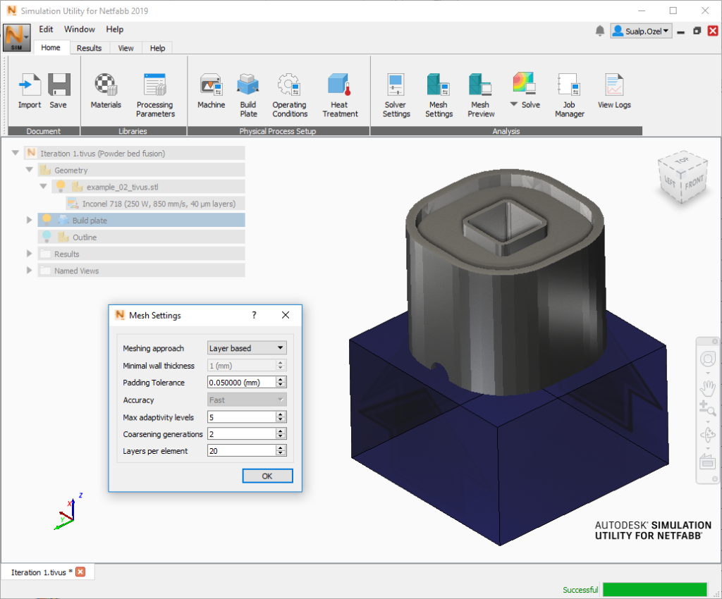
Figure 1: A “Layer based” meshing approach with varying “Coarsening generations” and “Layers per element” inputs were used to create the various iterations in this mesh study

Layers per element represents the number of powder layers in the thinnest element of the part. The size of the smallest element is equal to the Layers per element value multiplied by the powder bed layer thickness contained in the PRM file. A larger value of layers per element input produces a coarser mesh, and faster run time. Fewer layers per element are needed to represent small details, but both run time and memory usage may increase dramatically.

Coarsening generations is the maximum allowable number of coarsening steps taken. When coarsening is enabled, small elements are used to represent fine detail in critical areas, which is determined by the Layers per element control. Larger elements are used on the build plate and areas with lower detail requirements by combining smaller elements together, where the geometry allows. According to the Netfabb Simulation help documentation:

“A setting of 1 is generally a good compromise between speed and accuracy. Values of 2 or higher values should only be used for larger geometries that have large surface areas in the build plane, while also having fine features that need to be captured.”

In this study, I have used the Layers per element inputs ranging from 20 down to 5 and Coarsening generations inputs of 2 and 1 for the various iterations to test the impact of these settings on speed and accuracy.

Figure 2: Displacement, X (mm)  results from iteration 1 with a “Layers per element” input of 20 and “Coarsening generations” input of 2. All iterations are created using the same PRM file provided with the process parameter library included in Netfabb Simulation: Inconel 718 (250W, 850mm/s, 40 µm layers).

To determine when results have converged satisfactorily, I have used the following criteria:

• Display the Displacement result type, with the X component within the Plot settings
• Probe the X Displacement results along the same edge for each iteration during the same time step – as shown in Figure 3.

Figure 3:  The magenta nodes represent the edge probed for X displacement results for the time step at the end of the cooldown period, just before the substrate removal operation.

Model setup and computer specifications:

The model analyzed in this example is symmetric along the YZ plane as shown in Figure 3 above. Bounding box dimensions for the part is 32.12 mm x 32.12 mm x 25.4 mm in X, Y and Z directions respectively. In Netfabb Simulation, by default, the build plate dimensions would snap to the part boundaries. To avoid the edge effects this may cause on my part and to get more accurate displacement results, I increased the build plate dimensions to 40 mm x 40 mm in X and Y and kept it 25 mm in Z. I set the material for the build plate as SAE 304 and did not apply build plate heating. I also assigned a fixed boundary condition to the bottom surface of the build plate.

I ran all the iterations on my Windows 10 laptop with the following specifications: 4 cores (hyper treading turned off), 16 GB RAM. I chose this configuration as these are the minimum system requirements for Simulation Utility LT, which is included with Netfabb Ultimate, so that I can show the run times for a worst-case scenario configuration. I would highly recommend that you use a better computer when running your Additive Manufacturing Simulations to get faster results. Please refer to the recommended system requirements for running Netfabb Local simulation if you are trying to simulate production level models. Figure 4 below shows the mesh density details, whereas Figure 5 shows the run time differences between the 20 iterations.

Figure 4: This log graph shows the twenty iterations I ran for the same geometry. Iterations 1-16 utilized a “Coarsening generation” input of 2 and a “Layers per element” input ranging from 20 down to 5 with an increment of 1. Iterations 17-20 utilized a “Coarsening generation” input of 1 and a “Layers per element” input ranging from 20 down to 5 with an increment of 5.

After having run the first 16 iterations, it was clear that reducing the Layers per element input one at a time, while keeping all other meshing variables constant, did not have a significant impact on the overall mesh density until reaching iteration 8. Based on Figure 4 (above), I determined a more noticeable jump in the mesh density (Nodes and Layer.Nodes* count) can be observed when changing the Layers per element input by an increment of 5. That is why for iterations 17-20, I decreased the Layers per element input by an increment of 5.

*Note: Layer.Nodes are the number of simulated layer groupsmultiplied by the number of nodes of the final mesh.

Figure 5: This log graph shows the thermal and mechanical solve times for the 20 iterations. The thermal runs are typically 25% of the total time whereas the mechanical runs are 75% of the total run time.

The analysis times as shown in Figure 5 also correlated with my observation. To notice a significant change between iterations, I needed to change the Layers per element input by an increment of 5. Using this method, I saw a significant change in both the number of nodes and the run times as one can observe from the results of Iterations 17-20, which used Layers per element inputs of 20,15,10,5 respectively.

Now let’s look at the displacement results:

Figure 6: The X displacement results along the selected edge for the specified time step for iterations 1,6,11 and 16.

For clarity sake, I decided to present the results of iterations 1,6,11 and 16 in Figure 6. These iterations correspond with Layers per element inputs of 20,15,10,5 respectively with a constant Coarsening generations input of 2. Even though all four iterations capture the value of the largest displacement (~0.18 mm), the trend of X displacement is not properly captured with iteration 1. Iterations 6, 11 and 16 report similar trends for X displacement, but they have significantly different magnitudes for the local maxima (Z coordinate ~ 6mm) and local minima (Z coordinate~13 mm).

The inaccuracy in the trend of X displacement for Iteration 1 is significant as the compensation mechanisms used by the solver to create a warped shape rely on the displacement results of all the nodes, and not just the maximum displacement result.

Figure 7: The X displacement results along the selected edge for the specified time step for iterations 17,18,19 and 20

In the second half of my study, I decreased the coarsening generations from 2 down to 1 and created iterations 17,18,19 and 20. These iterations have the layers per element input of 20,15,10 and 5. Just as before, all four iterations properly capture the value of the largest displacement (~0.18 mm). But unlike Iteration 1 shown in Figure 6, the trend of X displacement is properly captured with iteration 17 (displayed in Figure 7). Figure 4 shows that these two iterations have roughly the same number of Nodes (and elements), but Iteration 17 has more Layer.Nodes. They also have relatively small run times as shown in Figure 5 (55 seconds vs 87 seconds)

Figure 8:  Side by side comparison of the internal mesh between iterations 1 and 20 with a clipping plane snapped to the global YZ plane.

So far, I presented the number of elements, run times, the change in displacement results and the more accurate capture of displacement trends going from one iteration to the next. With the images shown in Figure 8 (above), we can better visualize the change in the mesh density between the first and the last iteration in my study.

Iteration 1 mesh preview shows only a single element through the thickness, whereas iteration 20 has two to three elements through the thickness for all the thin sections in this model. Iteration 20 also does a much better job capturing the curvature of the model and it allocates more elements in the transition zones between the thin and thick sections of the model. All these factors play a critical role in obtaining an accurate solution.

What did we learn?

The key point in any mesh study is to ensure the results we get are accurate. If we do not perform a mesh convergence study, we will end up getting non-converged results.

In the case of additive manufacturing simulation, the incorrect results can manifest themselves as inaccurate maximum displacement results or inaccurate displacement trends. These displacements are typical input parameters used in decision making for part orientation, support structure planning, as well as compensated geometry creation. And as the saying goes: Garbage in, Garbage out!

This leaves you with one reliable option. Performing a mesh convergence study and making sure to compare the results of multiple locations consistently to check for convergence.

Although this example shows displacement results, the same method can be used to perform a mesh convergence study for temperature results.

Have questions? Comment below!

Until next time,

– Sualp Ozel, Product Manager

[1] NAFEMS, Open resources, Knowledgebase, The Importance of Mesh Convergence:  https://www.nafems.org/join/resources/knowledgebase/001/