In Finite Element (FE) modeling, the accuracy of any simulation is largely driven by the accuracy of the boundary conditions. In the modeling of Laser Powder Bed Fusion (LPBF) processes, the key thermal boundary conditions are:

Heat Input
Heat Losses
Mechanical Constraints

For now, lets focus on heat losses which occur during the LPBF process.

Heat Loss Mechanisms

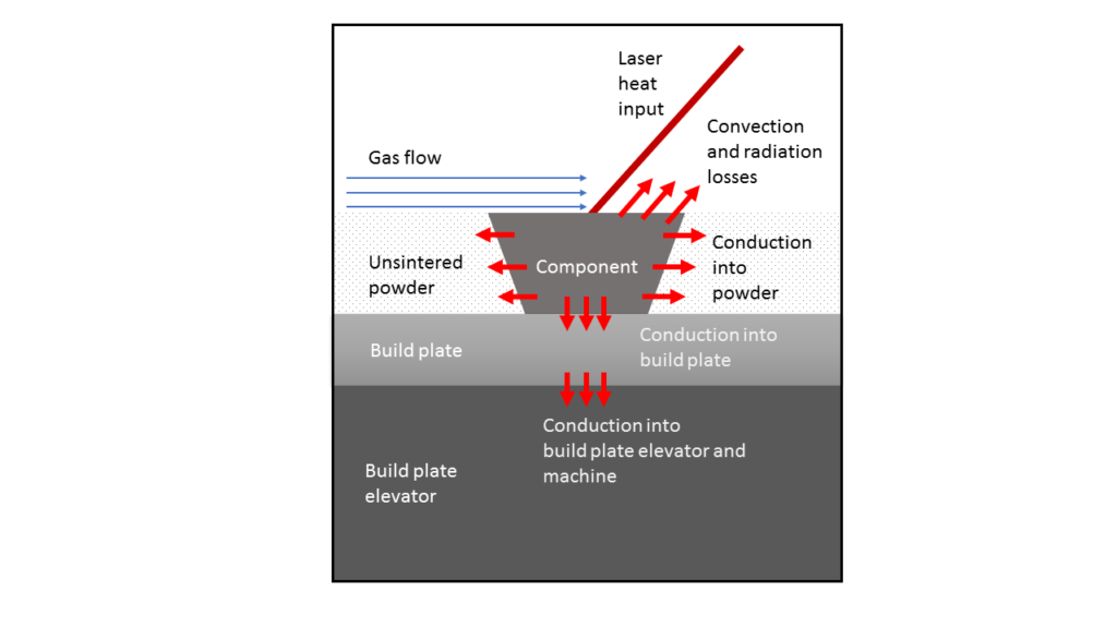
In LPBF, the heat input by the laser is conducted through the powder and component and is eventually transferred from the component and powder to the surrounding atmosphere and machine. This occurs by thermal radiation, free convection, and forced convection, as shown in Figure 1 below. Ultimately the heat absorbed by the LPBF machine itself is dispersed to the laboratory surroundings again by thermal radiation, convection, and conduction mechanisms.

Figure 1: Schematic showing heat transfer mechanism during laser powder bed fusion process

However, for efficient modeling, the entirety of the machine is impractical to include. Often, the entirety of the build plate is also too large to include in the FE mesh, as the build plate acts primarily as a heat sink in the thermal model and source of displacement constraints in the mechanical model. For similar reasons, the powder surrounding each build component is typically not included in the FE mesh as this can impose a large computational expense. As the unsintered powder, which surrounds components during LPBF process, has little impact upon the parts besides drawing heat away, it is common practice to approximate the heat loss into the powder as a surface heat flux. Yet there is still a question of how to reliably determine accurate heat flux values across a range of materials, as highly conductive powders, like Aluminum, will draw heat away at a much faster rate than a low conductivity metal, like Titanium alloys.

Material Based Heat Flux Calibration Methodology

One of the unique features of Netfabb Simulation is the ability to model powder directly in the FE mesh, due to the adaptive voxel mesher. This is used as a baseline simulation to determine most accurate heat flux for a range of thermal conductivities.

The methodology proposed to determine the relationship between the heat flux values and thermal conductivity is as follows:

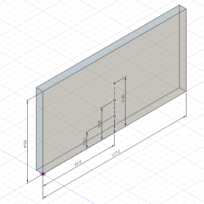
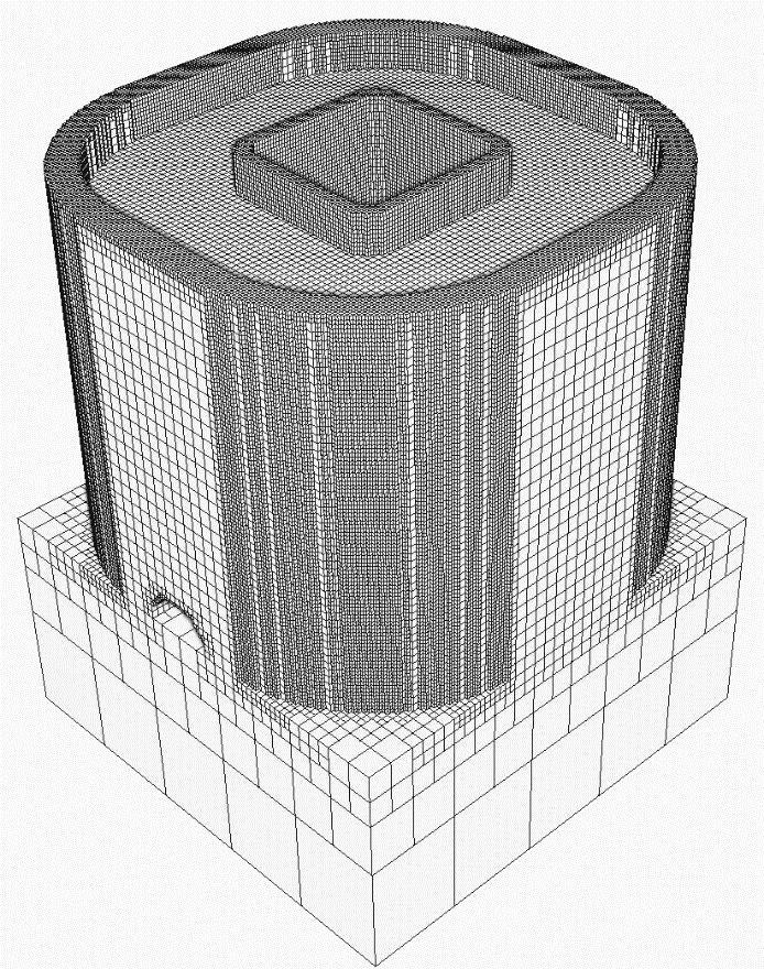
A set of thermal simulations for a wall shape are completed directly modeling the powder for materials of varying thermal conductivities. The materials tested were AlSi10Mg, Copper, Gold, Inconel 718, Platinum, pure Titanium, and Ti-6Al-4V. The test geometry may be seen in Figure 2.
A set of simulations are completed to determine the most accurate heat flux value for each material, using the direct powder models as reference. Temperatures are probed at heights of 13 mm, 25 mm, and 38 mm at the locations shown in Figure 2.
A regression analysis is performed to determine the relationship between thermal conductivity and calibrated heat flux values.

Figure 2: Example simulation geometry. All measurements in mm. The example geometry thickness is 6 mm. The vertical line shows profile for model comparisons.

Simulation Results

Example contour plots for the Ti-6Al-4V simulation are shown below. The heat flux for this model is set to 10 W/m² °C.

Figure 3: Convection approximation thermal results

Figure 4: Direct powder model thermal results

For each material the temperature profile along the center of the wall face are compared at 3 different heights along the face of the wall. A series of plots are made at each height to compare the different temperature profiles.

Figure 5: Example Ti-6Al-4V temperature profile comparison at 13 mm

Figure 6: Example Ti-6Al-4V temperature profile comparison at 25 mm

Figure 7 Example Ti-6Al-4V temperature profile comparison at 38 mm

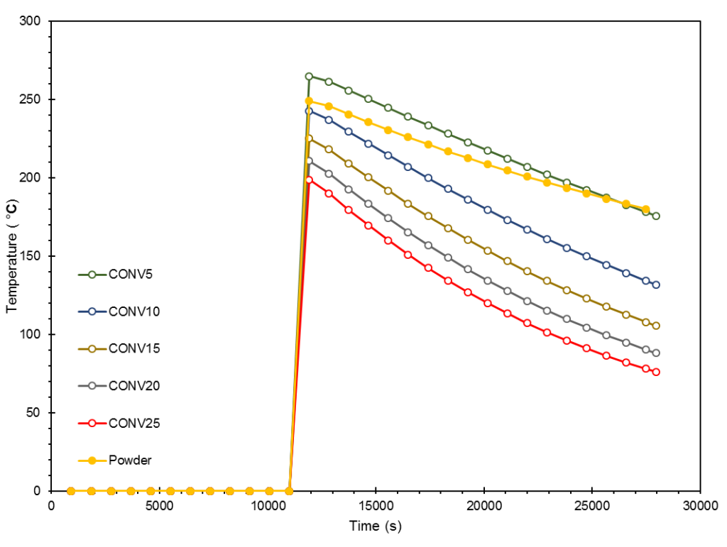
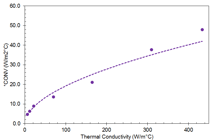
Examining these results, a heat flux value of 6 W/m² °C is likely to give the most accurate results for this material. This process is repeated for a range of materials of varying conductivities. From hundreds of simulations a relationship is built up between thermal conductivity and the closest convection approximation as shown below:

Figure 8 Correspondence between thermal conductivity and the approximated heat flux boundary condition

Integration into Simulation Utility for Netfabb

In the 2019.1 release of Simulation Utility for Netfabb, in the Operating Conditions dialogue there is a new option in the Thermal Boundary Condition dropdown, Estimated heat loss.

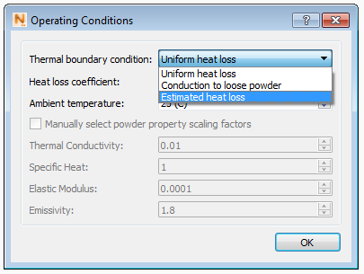
Figure 9 New estimated heat loss boundary condition

Selecting this option will have the solver query the select material’s room temperature thermal conductivity, and using the relationship shown in Figure 8, apply the most accurate heat flux value during simulation.

Conclusions

The accuracy of Finite Element simulations depends largely upon accurate boundary conditions. In the thermal modeling of Laser Powder Bed Fusion processes, meshing the powder directly gives accurate predictions of temperature, but requires a significant increase in mesh density. The higher mesh density in turn incurs a significant increase in RAM usage and computational time. Approximating losses to the powder as a constant heat flux is an alternative modeling strategy which requires far fewer elements to run, but it is difficult to determine what heat flux to use for each material. A set of simulations spanning very low to very high thermal conductivities discovered a relationship between the room temperature conductivity of a material and the most accurate heat flux approximation. This correspondence has been embedded into the FE solver and is available within Simulation Utility for Netfabb as an Estimated heat loss thermal boundary condition.

Material Based Heat Flux Approximations in the Finite Element Modeling of Laser Based Powder Bed Fusion

Heat Loss Mechanisms

Material Based Heat Flux Calibration Methodology

Simulation Results

Integration into Simulation Utility for Netfabb

Conclusions

Related Articles