The Low Poly Modifier Part 2

In Part 1 of this series, we looked at how to combine the Low Poly MCG modifier with a simple material graph to render scenes in a “Low Poly” art style.

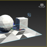
In this post, we’ll be taking a deeper dive into how this modifier was built. Along the way, we’ll be covering some useful TriMesh operators, and we’ll focus on how to work with random number generators. To get a bird’s eye view of what’s in store, here’s a little annotated timelapse of the Low Poly modifier being built:

In case you were curious, here’s a list of the main keyboard shortcuts I used in the video:

• Press “x” and type “*” followed by a keyword, for example: “*mesh”, “*color”, “*face”. This wildcard-based search helps me discover the operators related to a specific keyword.
• Hold “Ctrl” and drag a node onto a line to insert it. When your cursor is on the line, the line should appear as a dotted yellow line, indicating that the node will be inserted. I often use this technique with Pass-throughs to keep my lines nice and straight until I need them to curve into a portion of the graph.
• Hold “Shift” and drag your current selection to copy it.
• Press “Ctrl+S” and “Ctrl+E” to save and evaluate your graph.

We can split the “Low Poly” modifier into four major steps:

1. Setting the smoothing group of all the faces to 0.
2. Adding noise to the position of each vertex.
3. Coloring the face vertices such that: (a) faces pointing downwards (along -Z) are darker; (b) faces pointing upwards (along +Z) are brighter.
4. Optionally keeping the original vertices instead of the noisy ones for the final output.

1. Setting the Smoothing Groups to 0

You can compare this step to adding a “Smooth” modifier with no additional settings on top of an object. Setting the smoothing group of each face to 0 ensures that none of the faces are smoothed together. Conversely, if you wanted to smooth all the faces together, you could replace the Zero operator with a One (or a Constant of 1).

If you plan on working more extensively with the SetSmoothingGroups operator, it’s important to note that the integer values in the smoothingGroups array are interpreted in Max as individual bit arrays. Briefly put, if a face has a smoothing group value of 11 (represented in binary as 1011), this indicates that the face will belong to the first (1011), second (1011) and fourth (1011) smoothing groups on the mesh, and will be smoothed with the faces which also belong to at least one of those smoothing groups. For more information on this topic, look for the “Face Smoothing Groups” section here.

2. Adding Noise to Each Vertex

The second step is to change the orientation of each face by adding random noise to the position of each vertex. Alone, this step is responsible for giving planar geometry a slightly “crumpled” look, which is ideal for landscapes, rocks, trees, and foliage.

The noise is applied using a mapped function on all the vertices of the mesh. Once all the “noisy” vertices are computed, they’re applied back into the mesh with the SetMeshVertices operator. If you’re not acquainted with how functions work in MCG, I recommend you take a moment to get familiar with the concepts laid out in The Function Connector Part 1 – Reading MCG Functions.

At first glance, the noise function is a bit tricky to understand – it’s using a “Bind2of2” operator, and it seems to have two function arguments instead of just one. In fact, these two observations are related, and we’ll gently untangle why this is the case.

First off, one quirk of MCG is that a random number generator can’t simply be placed inside a mapped function. Doing so results in a brand new random number generator being created in every “loop”, giving the impression that the same random number is being applied to all the elements in the array. To show this, consider the following NoiseTest modifier, which connects a random number generator inside a mapped function:

With this construction, a new seeded random number generator is being created on every iteration, and is providing the same three values (which form the same “noise” vector) for all the vertices.

To resolve this issue, we need to modify the noise function to make it accept a generator as an argument. This way, we can bind the “generator” argument to a random number generator declared outside the function. This lets us use the same generator across all the vertices.

Here, the same generator can now continuously generate different values by advancing its own state every time a new random value is requested. This results in different random “noise” vectors being generated for each vertex.

Function argument binding is a more advanced (but very powerful) feature of MCG. When you bind a value to a function argument, the result is a new function that exposes one less argument. Here’s a visual breakdown of what’s going on:

After binding the “generator” argument, the new function will only have one argument left, namely the “vertex” argument. This is what we want, because we’re feeding an array of Vector3’s into the Map.

The last piece of this puzzle is why we are using the Bind2of2 operator instead of Bind1of2, or any other Bind operator. In this case, we need to use either Bind1of2 or Bind2of2 because we know our function exposes two arguments – the vertex (Vector3) and the generator (Random). If our function exposed three arguments, we would be looking for Bind operators containing the “of3” suffix, so our search would look like this: “Bind*of3”. Conversely, if the function exposed only one argument, we would just need to use the “Bind” operator.

Now that we’ve narrowed our options between Bind1of2 and Bind2of2, we just have to pick the right one. You could use the good old “trial-and-error” approach to see which one of these two operators makes your graph evaluate properly, however there is a more reliable way to tell which one to pick. I call this approach “Depth-First, Top-to-Bottom”.

Start at function’s output node, and step backwards through the graph, prioritizing depth first (i.e. “going backwards”), and then prioritizing the topmost connector you haven’t visited yet. Continue your “steps” until you’ve identified all the unconnected connectors. The order in which you find these connectors corresponds to the order of the function’s arguments. In the image above, we discover the “vertex” argument first, and then we continue our traversal until we discover the second argument. If you run into the same argument more than once, you can ignore it since it was already discovered in an earlier step.

The same binding technique applies to the Low Poly modifier’s noise function – we simply used the NoiseTest modifier to focus on the important bits of the concept. The main difference is that the Low Poly modifier has a slightly more elaborate noise function which:

1. Offsets and normalizes the random “noise” vector to ensure its domain lies between [-1,-1,-1] and [1,1,1], rather than [0,0,0] and [1,1,1]. This prevents all the vertices from “drifting” in a similar direction instead of moving around the vertex’s local position.
2. Decomposes the noise scale into three controllable parameters.

3. Coloring the Face Vertices

The third step involves coloring the face vertices based on the face’s orientation along the Z axis. Faces pointing upwards will appear brighter, with a color approaching [1,1,1], while faces pointing downwards will appear darker, with a color approaching [0,0,0].

For this section, one technical detail to keep in mind is that all the faces contained within a TriMesh are defined as triangles. As such, when we say that we’ll assign a color to a face, what we’re actually saying is that we’ll assign color values to all three of the face’s vertices. Colors in MCG are represented as vectors in the domain [0,0,0] (black) to [1,1,1] (white).

So, the idea here is to map an array of integers (which represent each face’s index inside the mesh) into an array of sub-arrays containing three colors. The three colors generated for each face correspond to that face’s vertex colors. The array of sub-arrays is then flattened, so that all the vertex colors can be applied into the mesh’s vertex color map channel.

Inside the mapped function, we’re taking the dot product of the face’s normal with the Z axis. If the normal points along the positive Z axis, the dot product’s value will be closer to 1.0. Conversely, if the normal points along the negative Z axis, this value will be closer to -1.0.

To rescale this value between 0.0 and 1.0 (which can then be used to define a color), we use an InverseFloatLerp with a minimum of -1.0 and a maximum of 1.0. This way, a dot product value of 0.5 will actually map to an InverseFloatLerp’d value of 0.75, while a dot product value of -0.5 will map to 0.25 (staying within the domain of 0.0 to 1.0).

4. Keeping the Original Vertices

The final step lets the user decide if he/she wants to keep the original mesh’s vertices instead of the noisy vertices in the final output. Regardless of the choice, the face colors will still be assigned as though the noise had been added. When the “Keep Vertices” parameter is enabled, the “true” branch of the If operator will be evaluated, otherwise the “false” branch will be chosen.

If you’ve powered through to this point, you should be well on your way to becoming an MCG expert! Feel free to post any questions or comments you might have! See you in the next post!

Download: LowPolyMod.zip

Instructions: Extract the file anywhere on your filesystem, then go to Scripting > Install Max Creation Graph (.mcg) Package, and select LowPolyMod.mcg in the extracted location. Once the package is successfully installed, it should appear in the modifier drop-down list.