When thinking of a frequency analysis, most people think of vibration. In this short blog, I’ll show you how using a ‘Normal Modes’ analysis in Nastran In CAD can provide you with valuable engineering insight into potential failure, and how the analysis can help with additional study types.
Most of us took high school physics and can refer to the standard tuning fork example. We would ping a tuning fork, and that tuning fork would produce two primary outputs: mode shape and excitation frequency. The same outputs provide us with critical information to understand the impact of resonance in our designs. Let’s assume we have a bracket mounted to a structure that has an operating frequency of a certain frequency. If our designs natural frequency coincides with the operating frequency, this will lead to a phenomena called resonance. The result of resonance is excessive displacements and high stresses that can lead to potential failure. In many aerospace applications, for example, high cycle fatigue due to vibration is the leading failure mode.
Although it’s critical for us to understand the aforementioned physics, we can also use a frequency analysis to debug other types of problems we run. In the image below, I ran an analysis on an assembly, where I eventually received a fatal singularity error. This error is referring to a lack of constraint in the model. In FEA, we must have stiffness in all three directions, or else there is what is referred to as a “rigid body mode”, where the body is completely free to move.
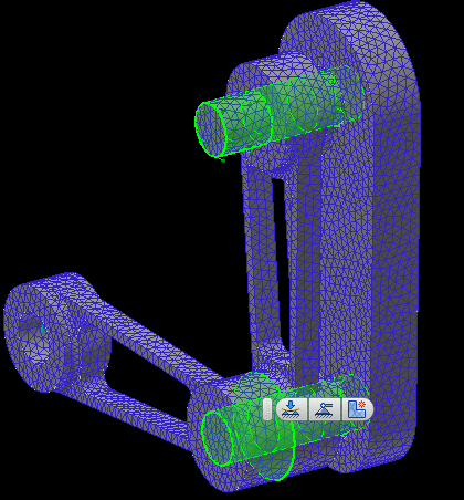
Figure (1): Static Analysis with Highlighted Contacts
Typically when I have an assembly with multiple bodies and not all faces are initially coincident, I will run a ‘Normal Modes’ study simultaneously. The reason for this is because the study will help identify regions where contact does not exist.
Clone your study (Duplicate) and edit the analysis type to ‘Normal Modes’. In the Modal Setup (shown in the image below, increase the number of output frequency to be six times the number of components you have in your study. The reason we prescribe six times the number of components is because there are six natural frequencies for every component (three rotations, and three translations), and also for main assembly structure.
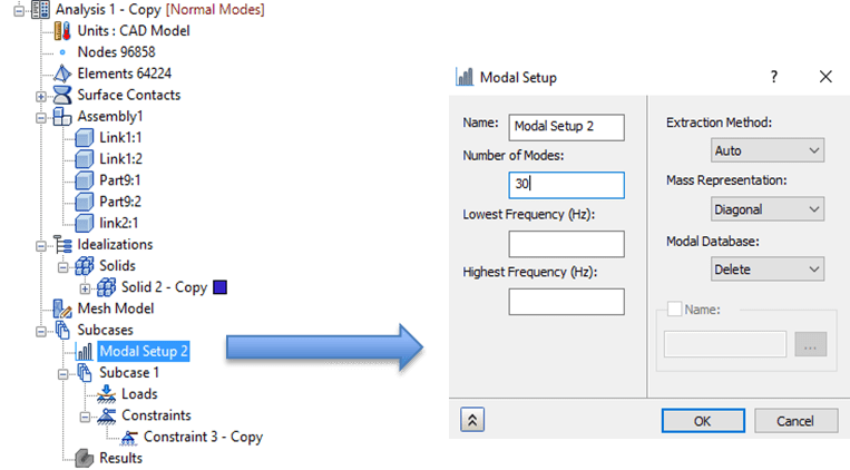
Figure (2): Prescribing Number of Output Modes
After running the study, observe the natural frequencies that are output in the analysis. If you observe a frequency value of near zero, there is a rigid body mode, and therefore, a lack of constraint. In the example below, my first natural frequency yields values of near zero for the first six natural frequencies. This means there is a lack of contact for a body in my analysis. Displaying the results will show you where that contact does not exist.
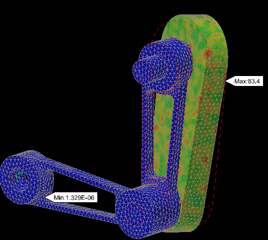
Figure (3): Modal Results of Rigid Body
Armed with this information, I can go to the contacts in the tree, and assign bonded contacts between bodies. After assigning this contact and re-running the analysis, my first natural frequency yields a value of 61 Hz and all bodies are constrained. I can now copy those contacts to the original analysis, and the study will run successfully.
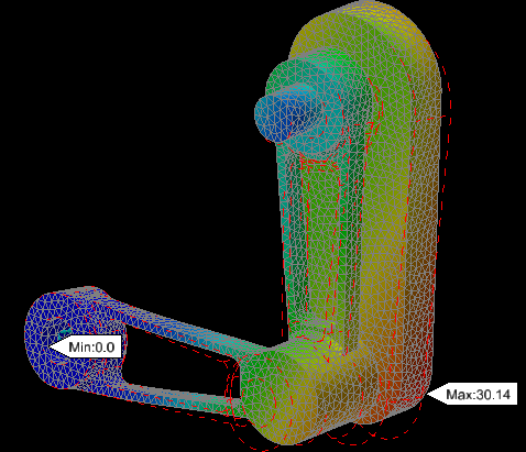
Figure (4): Modal Results with Fixed Contacts
Running a normal modes analysis not only provides us with valuable engineering information based off frequency values, but it can also be a great debug tool where there is a large amount of contact in the model.
Happy Simulating!

(0)