What is LMA and what can it do for you?
Local Mean Age, known as LMA, can show the amount of time the working fluid spends throughout the model – it can show which regions are stagnant and which are free-flowing. Below is an example of LMA being predicted in a pipe network where 3 types of pumping devices are employed:
- Axial fan
- Right cylinder blower with axial inflow and radial outflow
- Annular blower with radial inflow and outflow
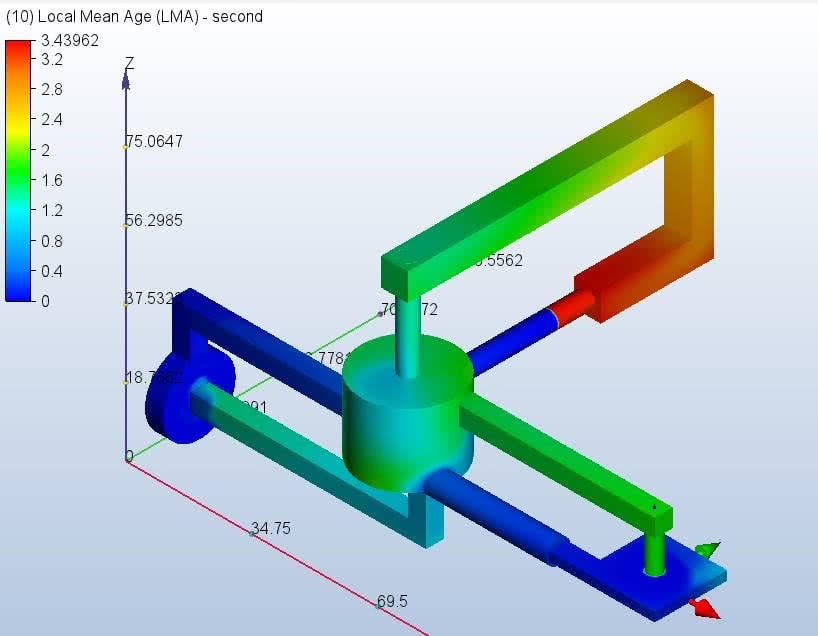
LMA = 0 BCs are automatically applied to the discharge faces of each pump. You can see the LMA values grow as we transverse each pipe loop. CFD2 computes the velocity field and CFD1 computes LMA at the intermediate save times and at end of run.
New and Improved
With our first update to CFD 2019, we’ve improved solution stability, solve times, and results capability.
Solution stability – changing from Implicit to Explicit solving:
Our original LMA equation looked like this:
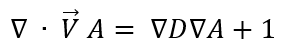
It can yield an ill-conditioned matrix, leading to long wall clock times to solve this matrix and, in some cases, the LMA solutions are so ill-conditioned that we cannot get a solution.
Adding an inertial term, the LMA equation now looks like this:
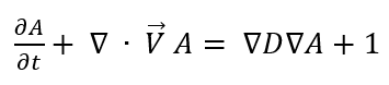
The advantage of using an explicit marching technique is that the ill-conditioned matrices are avoided, thus a solution is guaranteed.
Solve Times – Re-cast Explicit into an Implicit form:
The explicit solution of the LMA equations is quite time consuming – a small time step size must be used to insure numerical stability. We’ve explored multi-threading and, as a result, found that 10-15 threads can be employed optimally.
But this wasn’t the end of the story. Three things (the existence of a source term; the large element size ratios; and the unstructured mesh) make convergence difficult and here, we have all three. It was time for a new tactic – take the explicit discretized equations and re-cast them into an implicit form. The Implicit approach being applied to the explicit discretized LMA equations works pretty smooth.
This implicit form has many advantages:
- It is solvable. Convergence is not an issue since the 1/time step term can be used to control the diagonal dominance and the matrix condition number.
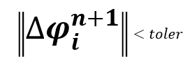
- Convergence can be computed using the L2 norm of delta phi.
- In this discretized form, the expense of forming the C matrix (advection + diffusion) is needed only once. The source term (1) and the diagonal addition (1/delta tau) are such simple forms that they can be computed on the fly and the LMA equation can be solved over and over again, modulating the time step size, until the LMA is steady.
Fortunately, the accelerant solver does not disturb the Cij matrix during the solve process, so it is perfectly suited to do many consecutive solves of our implicit form. With a controller to oversee the convergence of the LMA solution, we have a pretty good solution after 10 calls to the accelerant solver.
Results Capability – removing previous barriers:
In the original LMA code, there is logic to either compute LMA at every iteration or only at end of run. There was also logic allowing for extra “end of run” iterations, to assure that LMA is converged.
With the advent of the new LMA solver, those options are unnecessary and really don’t make sense. We are guaranteeing that we get a convergence solution every time we call the LMA solver, so extra iterations are unnecessary. Additionally, rather than worrying about every iteration versus just at end of run, it makes more sense to do the following:
- Update the LMA solution for each intermediate save point to include it in the *.res files.
- Guarantee that a LMA solution will update for the last iteration of a run, even when the stop button is employed or when the job stops due to auto convergence.
This ensures that the LMA field can be rendered at all visualization check points that are offered to the user. It also prevents wasting of CPU resources to compute the LMA at iterations where it cannot be visualized. This should save a lot of wall clock time, where in the past LMA calculations can dominate overall run times when they are computed at each iteration.
Because of these updates, we don’t have to support just end of run LMA calculations now – they are not that expensive, and we think it is more important to allow visualization of LMA coming from our *.res files. That eliminated flags, had clumsy controls, and makes LMA a special case. Instead, supporting intermediate saves and “end of job” saves gives the user the experience that is consistent with other field variables, such as velocity, pressure, etc.
The Bottom Line
LMA analyses are more accessible to you, enabling you to be able to achieve more reliable results with faster solve times, ultimately seeing your LMA solution evolve with your overall solution.
Just another way your CFD team is working for you
This post was done in collaboration with David Waite

(0)