For Background:
Meshing is the bane of any numerical analysis – what sort of mesh is appropriate? Autodesk CFD takes the guesswork out of this process via solution adaptive meshing in which the flow solution, rather than the user, orchestrates what the mesh should be. Repeated adaptation also leads to a mesh independent solution, the “pot of gold” for any numerical analysis. Furthermore, as the user community continues to tackle ever more complex models, associated meshes become larger making optimal meshes an absolute requirement for enhanced throughput and efficiency.
Mesh adaptation is comprised of three main elements:
- The calculation of adaptive mesh length scales
- The representation of that variation to the meshing processes
- The generation of the mesh based on that data
The efficiency of each of these processes is key to productive use of the technology. Feedback from the user community has, however, indicated that the computation of the length scales becomes particularly long for models larger than a few million elements. These reports prompted a second-look at this phase of the adaptation process.
Let’s Revisit:
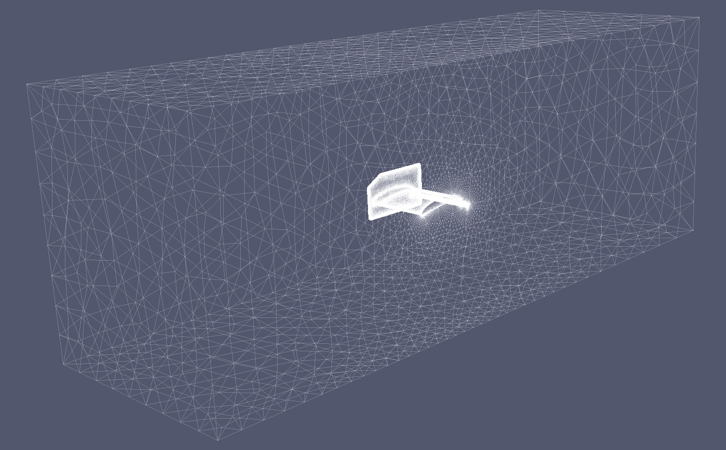
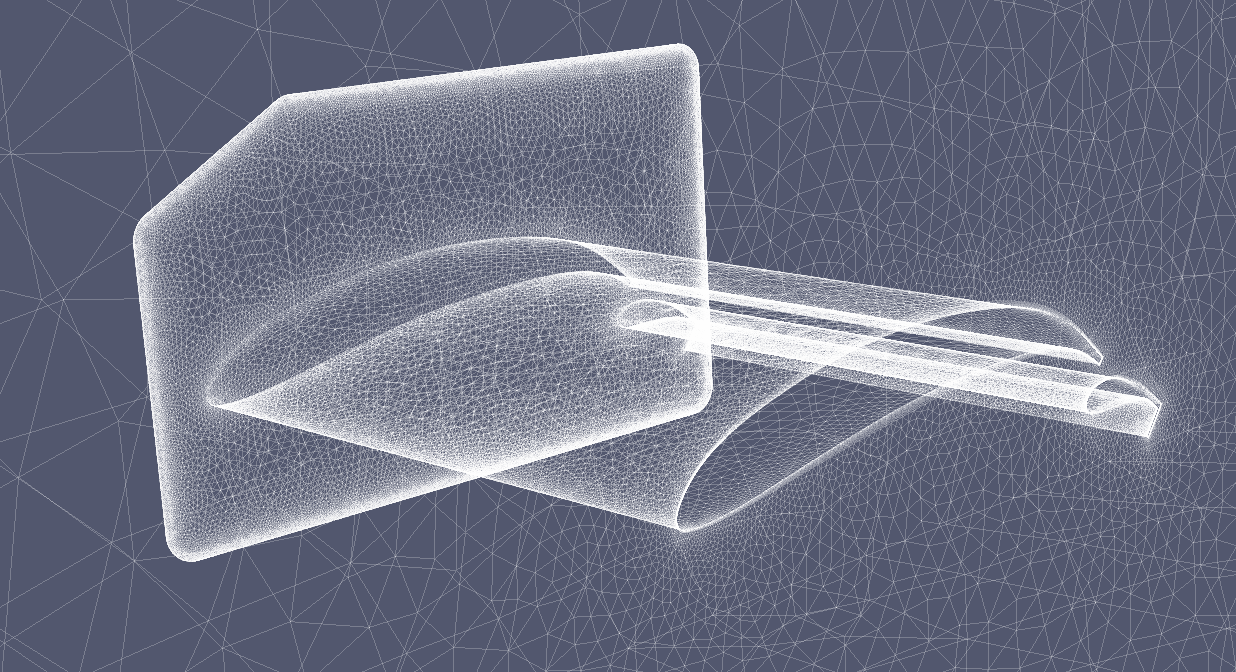
To benchmark the calculation of the adaptive length scales, a model of a spoiler configuration for an Indy race car was used as our test model. A baseline mesh composed of 7.8M elements and 1.3M nodes is shown below.
Calculation of the adaptive length scales is a multi-step process with the major elements consisting of:
- Calculation of the flow field derivatives (ui, vi, wi, Vi,j, Pi,j, and Ti,j)
- Solution error estimation & length scale calculation
- Length scale filtering
- Boundary layer mesh length scale adaptation and filtering
The resulting data resides within a spatial data structure, referred to as the background grid. Thread-safe query functions then expose the length scale variations to the surface, boundary layer, and volume meshing processes.
How bad is performance specifically? Process requirements and execution times for this model were observed as follows:
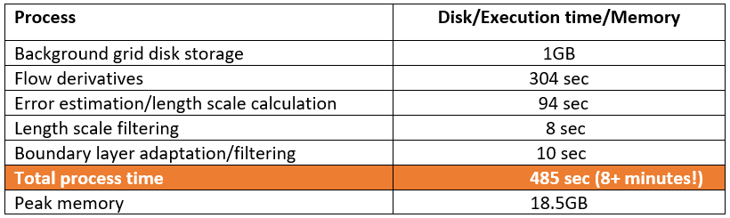
What the user is ultimately concerned with is the total process time, and 8 minutes for a model of this size is an eternity. Each process involved in these calculations was revisited with an eye towards a restructuring of the code and/or reformulation to introduce a threaded computation or enhance existing threaded performance. Efforts in each of these areas are described below.
Background grid disk space
Rather than leveraging the mesh object class as defined by the meshing library to serve as the background grid, a light-weight structure was developed that is not only more efficient in terms of disk space usage, but it is also sufficiently flexible to accommodate both manifold and non-manifold meshes, thereby providing support for simplified devices and other solver-specific mesh requirements not representable within the mesh object class.
Flow derivatives
The integration of the flow derivatives proceeds by element, and though the process had been threaded; even so, the lion’s share of the execution time is seen to reside within this process. A revision of the code to incorporate a more efficient container class, threading of the derivative initialization process, threaded import of flow field primitives, selective derivative evaluation (based on enabled adaptive error terms), and operation count minimization have led to significant gains in performance.
Error estimation & length scale computation
The error terms enabled within the calculation are a function of analysis type (flow and/or thermal) as well as other user-selected options. Their evaluation had been performed consecutively, with each requiring a sweep through the background grid. Threading was of little benefit in this process owing to the relatively simple formulation of each individual error term. An extensive revision involving the conversion of each error function to a point function now supports a single, threaded pass across the background grid, with an inner loop evaluating each enabled error function per background grid node. The ability to prescribe constraints on global refinement/de-refinement has also been added. These revisions have led to significant performance gains.
Length scale filtering
This process involves a threaded, recursive sweep across the background grid in which length scales may be adjusted to ensure a user-prescribed quality constraint is satisfied. Provisions for exempt and frozen nodes have been incorporated to support the presence of certain boundary conditions and simplified devices, respectively, as adaptive length scales are either evaluated owing to their proximity to other nodes or simply suspended to preserve existing length scales.
Boundary layer mesh length scale adaptation and filtering
The boundary layer length scales are adapted according to the nominal length scales so that the boundary layer mesh thins in accordance with the nominal length scales subject to a user-prescribed aspect ratio threshold and growth constraint. The calculation of the boundary layer length scales is also now threaded as is the follow-on filtering process.
The Result:
Using the revised approach, the performance improvements are as follows:
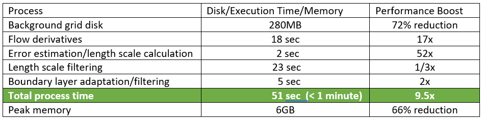
For the test model, we see a net speed increase of just under 10x in the calculation of the adapted length scales – reducing the eight-minute wait time to less than a minute. The increased efficiency, by which the adaptive length scales are computed, coupled with a threaded volume meshing option, yields a highly automated and efficient meshing process attractive to any user looking to optimize performance and throughput.
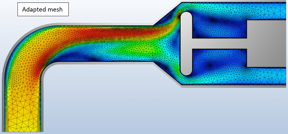
A Typical Result:
Solution adaptive meshing produces a result a user could not hope to duplicate manually, even with a priori knowledge of the flow field – and it does so automatically without user direction or intervention.
The model below demonstrates the capability of adaptive meshing. In this example the flow enters upwards from the bottom left, flows over the embedded obstruction, and exits at the right.
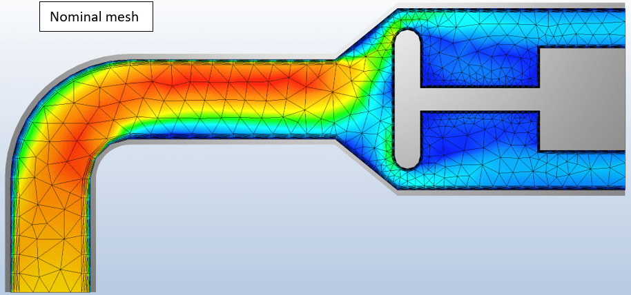
The adapted mesh captures the relevant physics including the shear layers, regions of flow separation and recirculation, and impingement areas.
In Conclusion
Use Mesh Adaptation to get the mesh you need without fussing about lost time, and with the latest improvements, now it will process even faster!
Be sure to stay up to date on releases and updates to take full advantage!
Thanks!

(0)