The United States and surrounding areas have experienced many tropical storms and hurricanes during the past few months. High winds put huge stress on infrastructure and can cause catastrophe if buildings, highways, signs, and other structures are not engineered to sustain the stress.
CFD can be used to predict wall forces on structures and therefore smarter engineering choices can be made. By using CFD you can understand “worst case scenario” environments and plan accordingly.
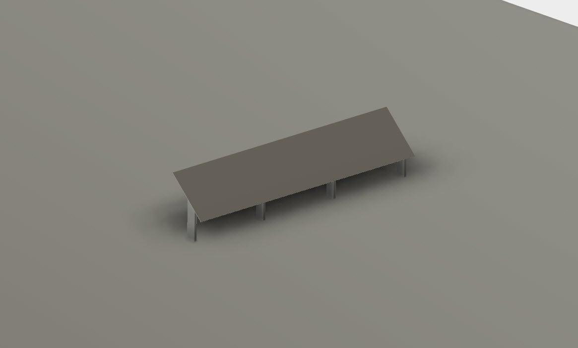
Here we have a solar array which is sustaining 150 mph winds. The panels are angled at 45 degrees and the wind is approaching the panels from the back. The solar array is 80.7 m^2 in area.
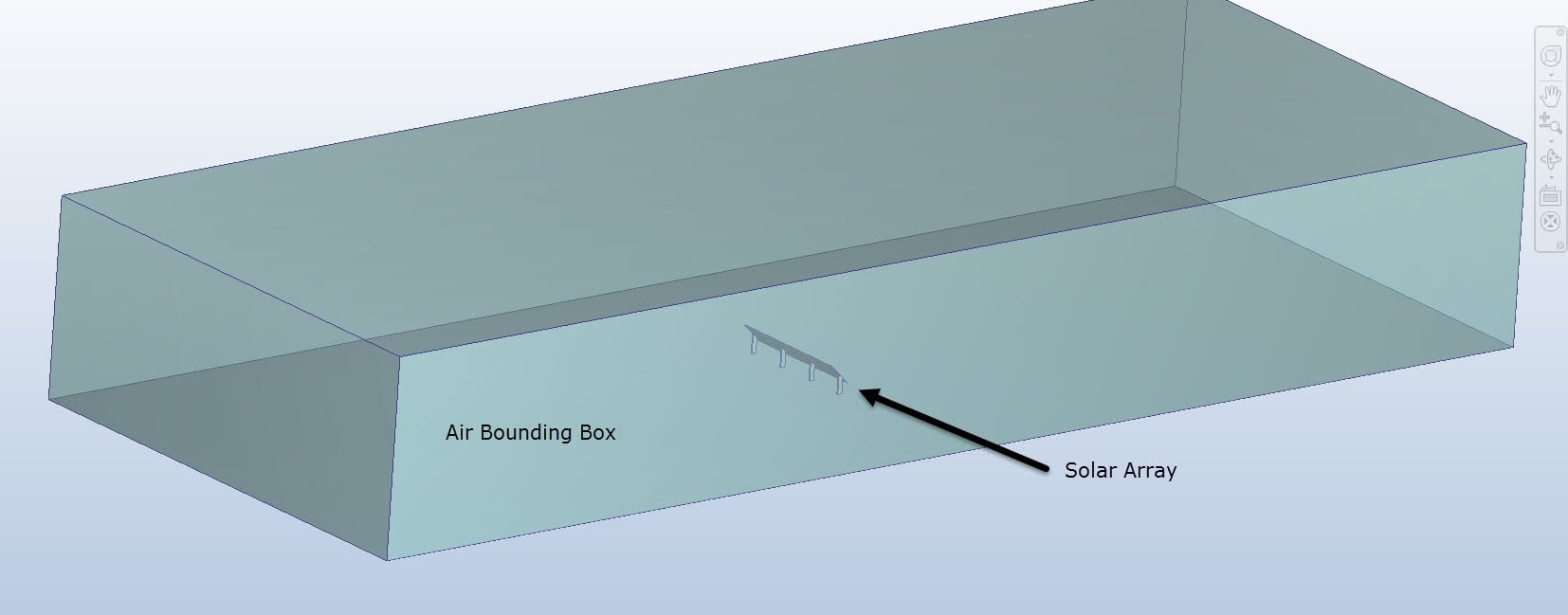
1.CAD Model:
The CAD model consists of the solar array and stands, and a large air volume domain. It is important to make the air volume large enough that the sides do no artificially limit the flow around the panels. A huge entrance and exit length allow steady, uniform flow to hit the solar array. Here the entrance and exit are both about 100 meters long- 5x the length of the solar array. There is about 1.5x length on each parallel side of the solar array, and the bounding box height is 30 meters high to allow for turbulence above the solar array.
Solar Array in CAD:
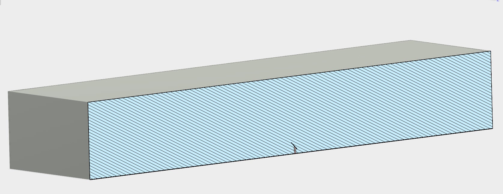
Section Analysis with Solar array in middle:
Materials:
This will be a flow only analysis; during a wind loading analysis we are not concerned with heat transfer.
Define the solar panels as steel
Define the fluid domain, or “bounding box” as air.
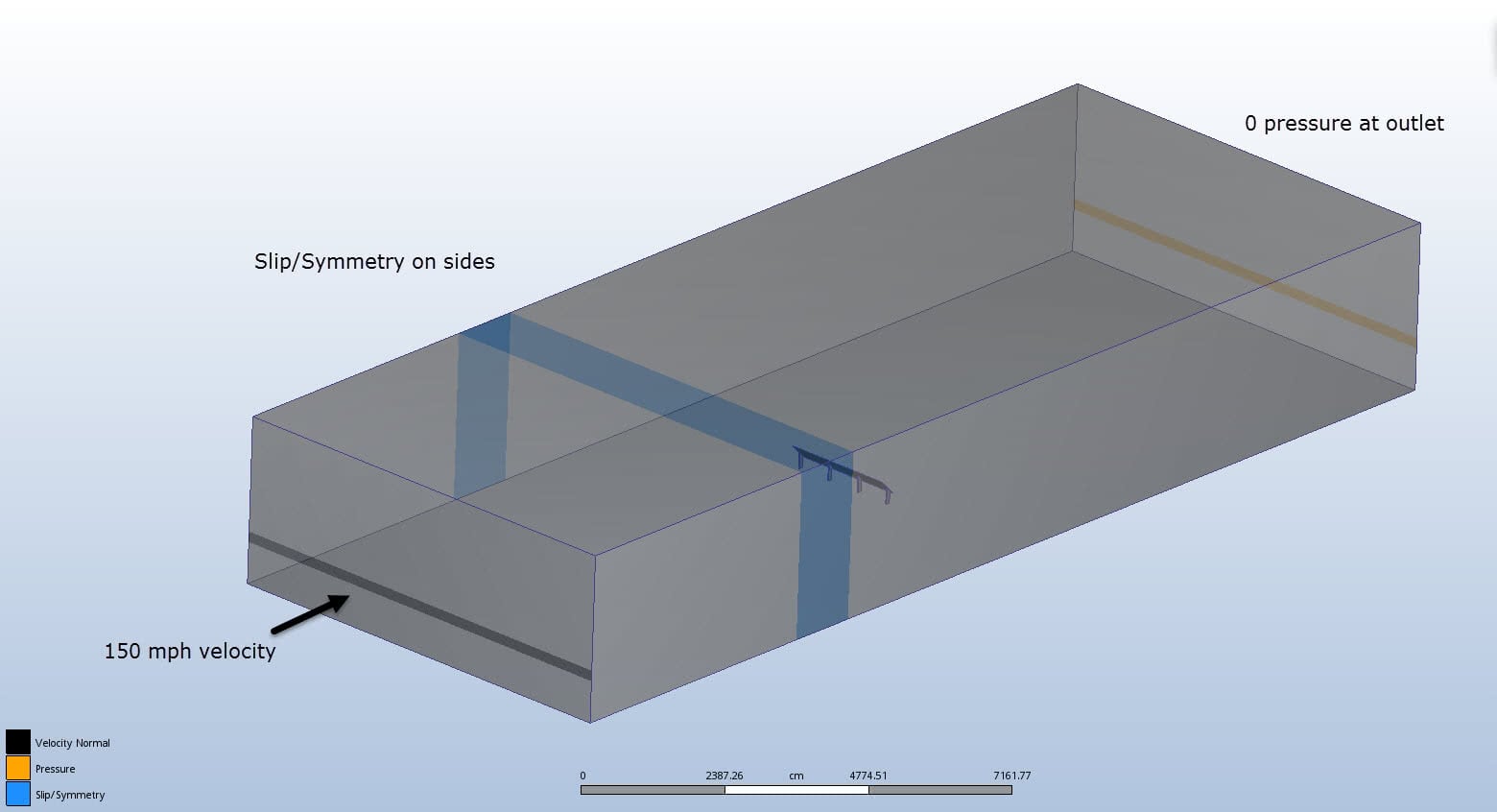
2.Boundary Conditions:
| Location | Boundary Condition |
| Inlet | 150mph |
| Outlet | 0 pressure gage |
| Front Side | Slip/Symmetry |
| Far Side | Slip/Symmetry |
| Top Side | Slip/Symmetry |
| Bottom | None |
The inlet side has a 150 mile per hour boundary condition. No temperature boundary condition is necessary because it is just a flow analysis- the solver will use standard temperature and pressure references.
The outlet has a 0 gage pressure boundary condition- this is standard of any CFD model outlet. The sides which represent “more air” and artificially constrain the side of the bounding box will use a Slip/Symmetry boundary condition. This means the velocity of the fluid at the wall is the same as the free stream velocity- the wall will not artificially slow down the flow via a boundary layer.
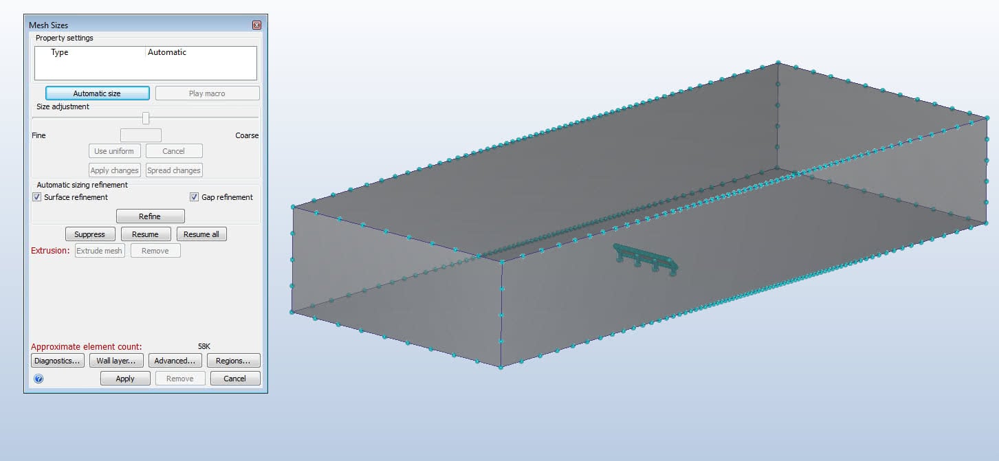
Meshing:
An automatic mesh with Surface and Gap refinement was used for this model. After an initial autosize, the sizing was refined by selecting the air domain and changing the Size adjustment bar to 0.5. 5 wall layers were used to better capture the flow shedding off the solar array.
Automatic Mesh:
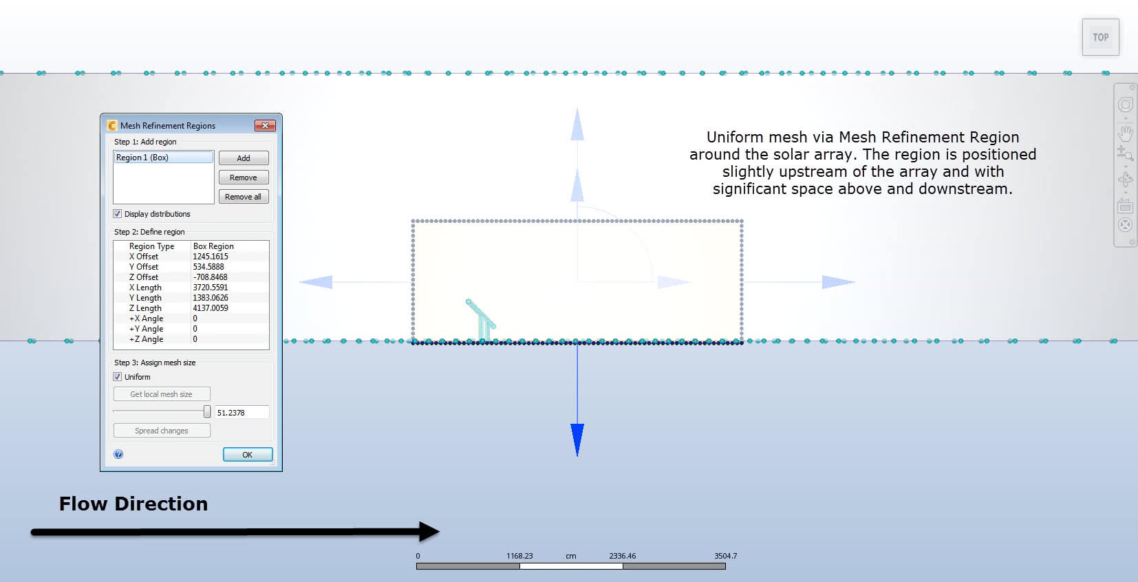
A Refinement Region is used around the solar array. This region will have a uniform mesh by default and needs to be very dense in order to capture the flow around the array. The region will automatically assign an element size equal to the smallest edge length within the box. This can be changed, but it is generally a great starting point.
Refinement Region:
Solve:
On the Solve dialog, set the solution to Steady State and run for 1000 iterations. The solver will assess convergence automatically and will stop when a final solution is obtained. Use the SST K-omega turbulence model, which can be set via Physics>Turbulence. This will capture shedding of flow off the solar panels better.
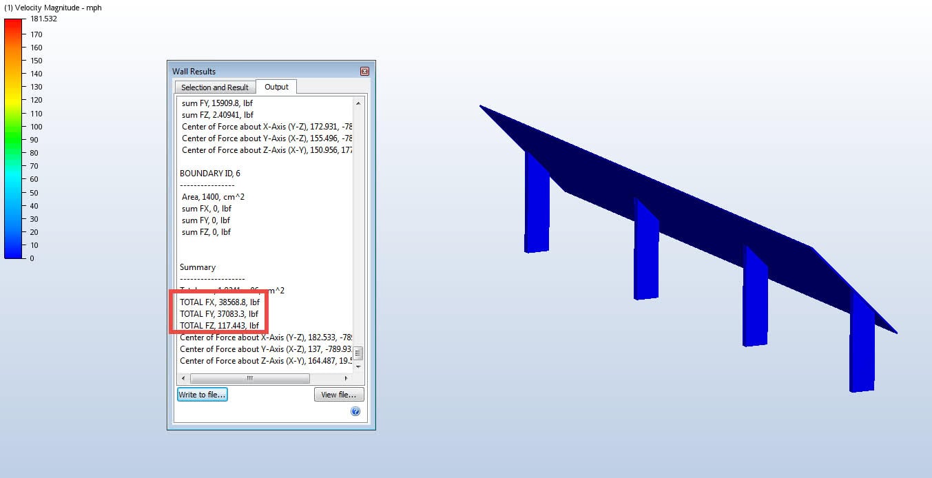
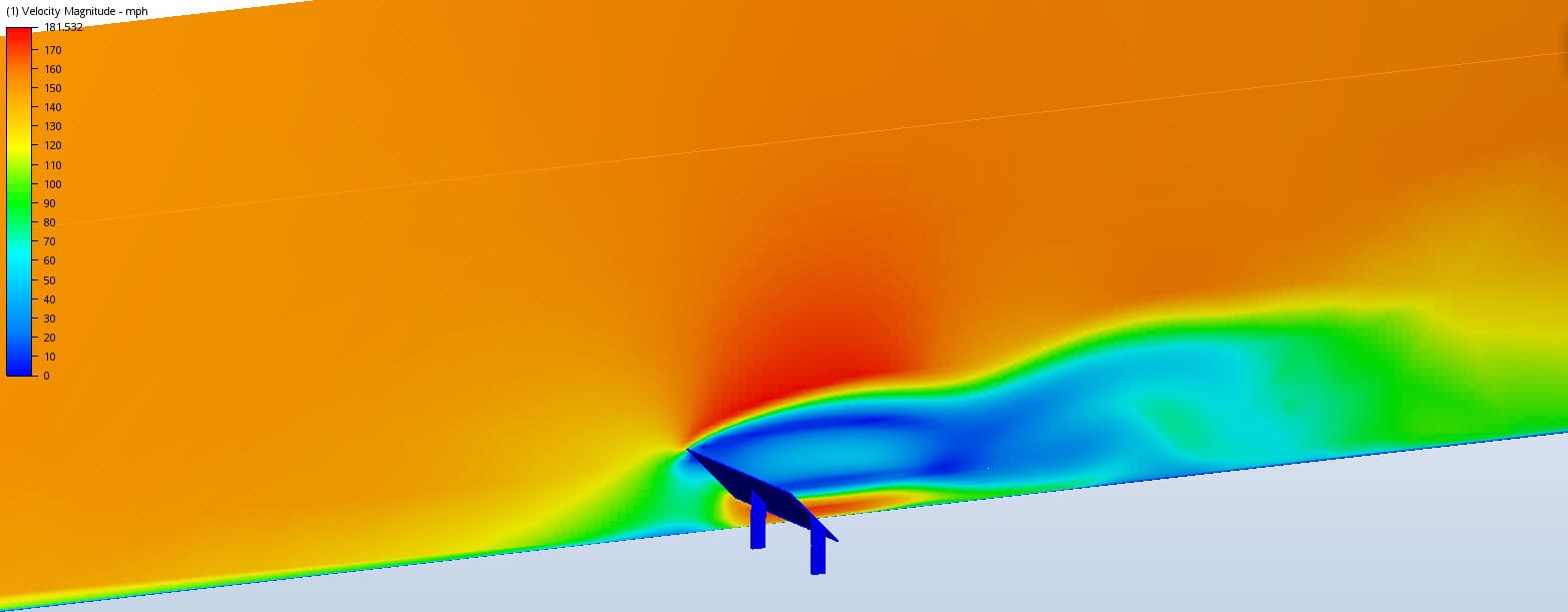
Results:
Cut planes and traces can be used to better understand the flow around the solar array. The Wall Calculator can be used to look at wall forces on the array. Here we can see the total drag in the flow direction, Fx, is 38,568 lbf and the total lift is 37,083 lbf. Clearly it is critical this structure is mounted in a safe and strong fashion.
Velocity Cut Plane:
Wall Calculator: