Background:
Our development team works behind the scenes on many of your support cases and the other day, our technical support team shared a customer case with us that was slow to solve – as in 24+ hours slow. YIKES! Time for a deep dive into the code.
Dev team to the rescue!
The analysis had several Distributed Resistance (DR) volumes and the ratio of DR elements / Fluid elements was high. 44M elements made up the fluid volume and the time spent set up the DR flow length estimates within the DR parts was ~24 hours. The DR FLM (flow length model) is a model where the resistance length is computed from the DR part geometry. The process of computing the resistance length goes as follows,
1. Assign group numbers for each unique inlet and outlet for the DR parts.
2. For each DR fluid element of a DR part, compute the distance to the closest two group surfaces.
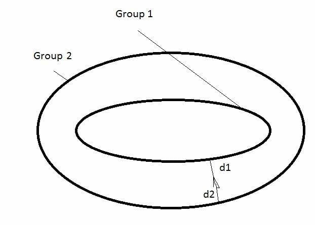
D1 measures the closest approach point to group 1. D2 does the same for group 2.
This process is very computationally intense since we have a M x N distance computation, where M = elements that make the DR volume and N = DR surface element faces making up the inlet and outlet surfaces.
Initially, we rewrote the algorithm to do this in such a way as to minimize the operation count. Performance tests revealed that we could reduce the DR initialization time some, but we were really not putting enough of a dent in that massive 24-hour compute.
The main limitation to speeding up this calculation was the fact that the algorithm was running on just the CFD1 master process. Study of the original algorithm reveals that it is a perfect candidate for multi-threading. This is because all the data used in the computation is of global scope. What this means is that multiple threads can read this global scope data without contention (no mutexting required). And the same is true for the writing of the output vector of DR lengths since DR element lengths are sequentially loaded without any assembly process.
To accomplish the multi-threading of the master process, we first constructed a procedure that tests how many threads we can use effectively. First, we define a dense computation like,
result = 0.;
for (i = 0; i < 1000000000 / opt_threads; ++i)
result += sin(i / 100.) + cos(i / 1000.);
if (!tid)
printf(“result %f\n”, result);
In the for loop, each thread executes 1000000000 / opt_threads times. We call this computation and vary the value of opt_threads and record the execution times,
Next we compute threading efficiency, wct[1] / (wct[N] * N), where N is thread count N and wct is wall clock time recorded at each thread count.
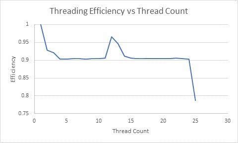
Notice the drop-in performance at 25 threads. This is expected since the test was run on a desktop machine that has 24 cores. So, in a few seconds we can automatically determine the optimal thread count, just by locating this performance drop off point.
Next, we placed the DR distance search algorithm into the same multi-threading environment (which required very little modification from the original source code due to the fact that so much of that code references global scope variables.) At this point, you have two options.
1. Direct each thread to compute the DR lengths in element blocks.
2. Process the whole list of elements and assign a unique element id to each thread.
Option 1 is only good if you can apriori parse out the work load per thread equally – in this particular case, we cannot. So, option two is handled by mutexting the element index and sequentially assigning that index to each thread as they enter the mutext zone. Mutexting assignments in this way is very effective and yields perfect load balancing. Luckily, mutext assignments occur in the micro second time scale.
The first test we ran was using a 4-core laptop.
Original algorithm running on master process = 88950 seconds
New algorithm running on 4 threads = 15768 seconds (speed up = 5.64X ).
The speed up is better than 4X by virtue of the minimization of operation count work we did earlier.
Next, we ran this on a 24-core desktop. Here is speed up as thread count is varied
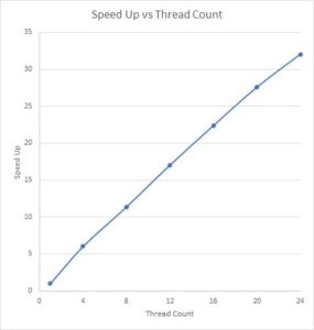

Using 24 threads shows 100% CPU utilization.

While we work to speed up the CFD1 initialization process, it is important to note that this multi-threading of the master process can be extended in several ways:
1. Any master only computation that computes a dense kernel which involves primarily global memory access to array data and non-contentious memory writing for outputs can utilize the threading code developed here. In fact, the thread wrapper is written in the following form to allow it to be extended to other procedures.
- case 0: Determine optimal thread count via a timing study
- case 1: Compute dense kernel 1 – DR resistance flow length
- case 2: Compute dense kernel 2 – ?
- case 3: Compute dense kernel 3 – ?
2. There are instances in CFD1 where the 0 rank slave process computes dense kernels. The threading code developed here can be extended to the 0 rank MPI process (or any other MPI process – which is essentially the design of CFD2).
It is important to note also that any optimization you do in your code that minimizes operation count, is multiplied by your thread count.
The Net Result:
In this example, we got a 1.333 speed up on a single thread just by re-writing the source code to minimize the operation count. When running 24 threads, we see the speed up increase to 24 * 1.333 = 32X. Here’s your CFD team is working for you!
Be sure to update to CFD 2019 this April to be sure your Distributed Resistance analyses will run fast too.
This post was done in collaboration with David Waite

(0)